
After weeks of staring at policy gradient equations, Bellman optimality conditions, and exploration-exploitation tradeoffs, you’re no closer to knowing which RL algorithm to use for your robotic arm. The textbooks cover the theory beautifully, but when you sit down to pick an algorithm for your actual robot, that theoretical knowledge feels distant and abstract.
You’re not alone. The gap between RL theory and robotics practice is real, and it trips up even experienced engineers. Theory teaches us about optimal policies in infinite time, but your robot needs to learn grasping in 200 real-world trials. Papers showcase algorithms on simulated benchmarks, but your hardware has sensor noise, calibration drift, and a habit of breaking when it explores too enthusiastically.
This article offers something different: a decision-driven framework for selecting RL algorithms based on your actual constraints. Instead of starting with “here’s how PPO works,” we start with “what does your robot need to do, and what resources do you have?” We’ll walk through the key decision points that matter in robotics, observability, dynamics knowledge, sample budgets, and safety requirements, and map them directly to algorithm families.
Think of this as a practical field guide. We’ll use a decision diagram as our map, work through concrete robotics scenarios, and focus relentlessly on the questions that matter when you’re implementing RL on real hardware. By the end, you’ll have a systematic way to narrow down the algorithm space and make informed choices for your specific problem.
The RL Algorithm Decision Framework
The overwhelming thing about RL isn’t algorithmic complexity; it’s the sheer number of options, and the theory doesn’t tell you when to use which one. You need a navigation tool that respects real-world constraints.
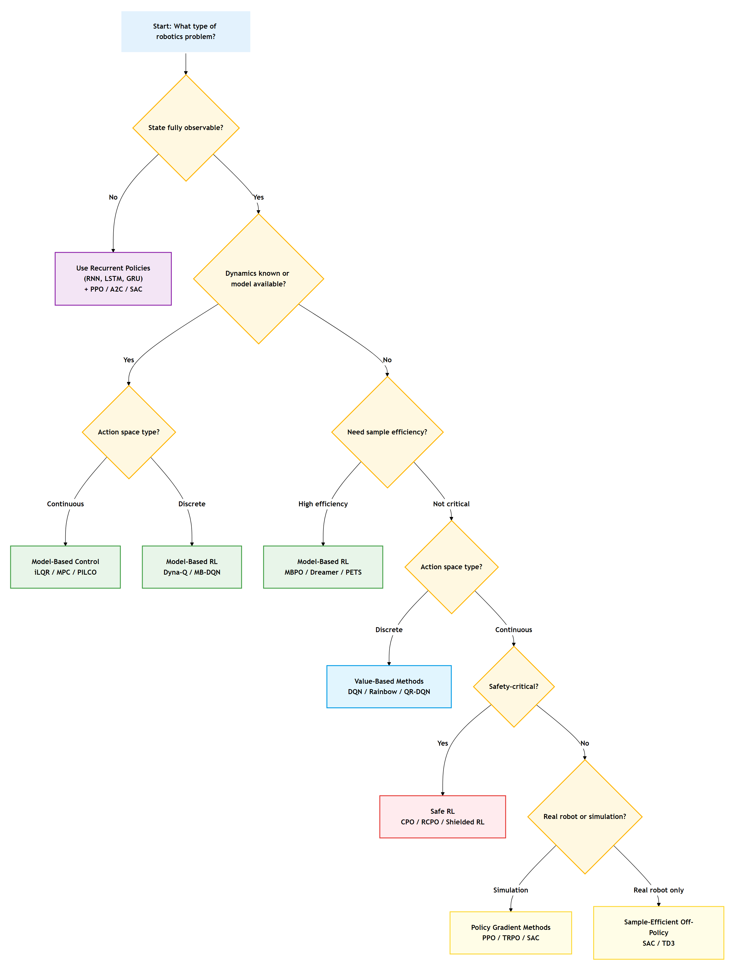
The decision diagram below is that tool. It works by asking questions about your robotics problem that you can actually answer: Can your sensors fully observe the state? Do you have a dynamics model? How many real-robot samples can you afford? Each branch leads you toward algorithm families suited to your constraints.
This isn’t a perfect oracle; real problems are messy and often need hybrid approaches. But it gives you a structured starting point instead of analysis paralysis. Let’s see the map, then walk through each decision point.
Key Decision Points for RL Algorithm Selection
Let’s unpack each fork in the decision tree. These aren’t abstract theoretical distinctions; they map directly to hardware limitations, budget constraints, and safety requirements you face in real robotics projects.
Is Your State Fully Observable?
This question asks: can your sensors tell you everything relevant about the world right now, or do you need to remember the past?
In robotics, full observability is rarer than you’d think. A camera-based grasping system can’t see the back of an object. A mobile robot might not know whether a door is locked until it tries to push it. A manipulation task with contact requires inferring forces from indirect measurements. These are all Partially Observable MDPs (POMDPs).
When the state isn’t fully observable, your policy needs memory. Recurrent neural networks (RNNs, LSTMs, GRUs) let your policy maintain an internal belief state based on its observation history. You pair these architectures with standard RL algorithms, such as PPO with LSTM policies or SAC with GRU encoders.
The practical cost? Training becomes slower and less stable because you’re learning both a policy and a state estimation strategy. But if your problem genuinely has a hidden state, no amount of clever feature engineering will fix a memoryless policy.
Do You Know the Dynamics?
This is the model-based versus model-free divide, and it’s huge for robotics.
If you have a dynamics model, whether from physics equations, a simulator, or a learned model, you can plan. Model Predictive Control (MPC) solves optimization problems online using your model. For continuous control with known dynamics, methods such as iLQR or DDP often outperform model-free RL in terms of sample efficiency and performance.
Consider quadrotors: their dynamics are well-understood in terms of rigid-body physics. You can write down the equations, and MPC works beautifully. But manipulation with contact? Those dynamics involve friction, deformation, and discontinuities that are notoriously hard to model accurately.
Model-free RL shines when dynamics are too complex to model or when you want to avoid model bias. PPO, SAC, and TD3 learn directly from experience without assuming a dynamic structure. The trade-off is sample complexity: model-free methods typically require orders of magnitude more data.
The middle ground is model-based RL: learn a dynamics model from data, then use it to improve sample efficiency. We’ll cover this in the algorithms section.
Action Space: Discrete or Continuous?
Your action space determines which algorithm families are even applicable.
Robotics deals with continuous control of joint torques, velocities, or positions, so value-based methods like DQN are unsuitable for these real-valued vectors. Instead, use policy gradient techniques (PPO, TRPO) or actor-critic algorithms for continuous action spaces (SAC, TD3).
But not all robotics problems are continuous. High-level task planning might choose from a set of discrete waypoints. A gripper might select grasp candidates from a finite set. Mobile manipulation could involve discrete mode switches (navigate, manipulate, inspect).
For discrete actions with known models, classical planning or model-based RL (Dyna-Q, Model-Based DQN) works well. For discrete actions without models, DQN variants are your go-to. The key is recognizing when discretization makes sense versus when it throws away critical information.
Sample Efficiency: Can You Afford to Learn?
This might be the most important question for real robotics.
Simulation benchmarks report algorithms running for millions of steps. Your real robot? Maybe you can afford 100-500 trials before wear, time costs, or supervision requirements make it impractical. Sample efficiency isn’t a nice-to-have; it’s often the constraint that determines feasibility.
Model-based methods generally outperform other methods in terms of sample efficiency. MBPO learns a dynamics model and generates synthetic rollouts for training. A Dreamer learns in the latent space to handle high-dimensional observations. PETS uses ensembles for uncertainty-aware planning. These approaches can learn meaningful behaviors in hundreds rather than tens of thousands of episodes.
The catch is model error. If your learned model is wrong, the policy will optimize for the wrong dynamics and fail on the real system. Model-free methods are less sample-efficient but more robust to this model bias.
In practice, many robotics applications use simulation for the bulk of training (to address sim-to-real transfer challenges) or start with model-based methods and refine them with model-free fine-tuning.
Safety: What’s the Cost of Failure?
Standard RL algorithms explore by trying potentially dangerous actions. That’s fine in simulation, less fine when your robot costs $100K or operates near humans.
Safe RL adds constraints during learning. Constrained Policy Optimization (CPO) and its variants enforce safety constraints in expectation; the policy isn’t allowed to violate constraints on average. Shielded RL uses a verified safety controller that can override the learned policy. Recovery RL trains separate policies to handle constraint violations.
The robotics applications where this matters most: surgical robots, human-robot collaboration, expensive hardware, or any system that requires safety certification. You accept slower learning in exchange for guaranteed constraint satisfaction.
Even if you’re not using formal safe RL, thinking about safety early matters. Simple approaches like reward shaping to penalize dangerous states, careful action space limits, or using simulation to pre-filter obviously bad policies all help.
The Algorithms That Matter in Robotics
Now that we’ve mapped out the decision points, let’s examine the specific algorithms that emerge from this framework and how they perform in real robotics contexts. This isn’t comprehensive; it’s focused on what works in robotics practice.
Policy Gradient Methods (PPO, TRPO)
These algorithms directly optimize the policy using gradient ascent on expected reward. PPO (Proximal Policy Optimization) clips updates to prevent destructively large policy changes. TRPO (Trust Region Policy Optimization) enforces this more rigorously with a constraint.
They’re on-policy: they use only recent data, which makes them less sample-efficient but more stable. PPO has become the workhorse of robotics RL because it’s robust, easy to tune, and works reliably across diverse problems.
When to use them: You have access to good simulation, can afford moderate sample requirements (thousands to tens of thousands of episodes), and want stable, reliable learning. Robotics wins include quadruped locomotion (ANYmal, Cassie), dexterous manipulation, and drone acrobatics.
The key hyperparameter is the clipping threshold (typically 0.2), and you need careful normalization of observations and rewards. But once tuned, PPO is remarkably reliable.
Off-Policy Methods (SAC, TD3)
These algorithms learn from old data stored in a replay buffer. SAC (Soft Actor-Critic) maximizes both reward and entropy for robust exploration. TD3 (Twin Delayed DDPG) uses two Q-networks and delayed policy updates for stability.
Sample reuse makes them more sample-efficient than on-policy methods. This is crucial for real-robot learning where every trajectory is expensive. You can also mix simulation and real data in the replay buffer.
When to use them: Every real-world sample is precious, you’re doing online learning on hardware, or you want to fine-tune a sim-trained policy with real data. Robotics wins include real-world manipulation learning, fine-tuning for unmodeled dynamics, and continuous improvement from operational data.
SAC is generally preferred over TD3 for its automatic temperature tuning and better exploration. Both require careful tuning of critic learning rates and target update frequencies.
Model-Based RL (MBPO, Dreamer)
These methods learn a dynamics model, then use it to generate synthetic training data or plan in imagination.
MBPO learns an ensemble of dynamics models and generates short synthetic rollouts to augment real data. Dreamer learns a world model in latent space and trains policies entirely in imagination. PETS (Probabilistic Ensembles with Trajectory Sampling) uses uncertainty-aware planning with model ensembles.
When to use them: Sample efficiency is critical, you can afford the complexity of training models, and your dynamics are learnable (not too stochastic or chaotic). The challenge is that model errors compound, and small prediction errors lead to large policy failures.
In robotics, model-based methods shine for problems like manipulation with limited real data, where you can learn object dynamics models and use them for planning. They’re less common in production than model-free methods because of the compounding error problem.
Safe RL (CPO, RCPO)
These algorithms optimize reward subject to safety constraints. CPO extends TRPO with constraint satisfaction guarantees. RCPO provides more robust constraint satisfaction.
They work by maintaining a constrained budget during policy updates, ensuring that the expected cost stays below a threshold even while maximizing reward. The policy might learn more slowly, but it won’t violate critical safety bounds during training.
When to use them: Physical safety matters, constraint violations are unacceptable, or you need certified behavior. The tradeoff is slower learning and additional complexity in specifying constraints as expectations over trajectories.
Robotics applications include human-robot interaction (guaranteeing human safety), delicate manipulation (force limits), and anywhere you need formal safety arguments for deployment.
RL Algorithm Selection: Real Robotics Scenarios
Theory is great, but let’s see how you actually use this framework on concrete robotics problems.
Scenario 1: Robotic Grasping
You’re building a bin-picking system. A single RGB-D camera looks at a bin of objects from above. The robot must grasp objects despite occlusions and sensor noise.
Walking the diagram: The state isn’t fully observable (can’t see the bottoms or backsides of the objects). You don’t have accurate contact dynamics models. Your action space is continuous (end-effector poses or joint commands). Sample efficiency matters. You want to learn on the real robot with hundreds, not thousands, of grasps.
The path leads you to: Recurrent policies (LSTM to handle partial views) + SAC (continuous control, sample-efficient off-policy learning). You’d likely start with a sim-trained base policy using domain randomization, then fine-tune on the real robot with SAC, collecting real grasps into a replay buffer.
Why this works: The LSTM tracks belief about hidden geometry. SAC maximizes sample reuse from expensive real grasps. Entropy regularization encourages exploration of diverse grasp strategies.
Scenario 2: Quadruped Locomotion
You’re training a quadruped robot to walk over rough terrain. You have a physics simulator (MuJoCo or PyBullet) and joint encoders that provide full state.
Walking the diagram: State is fully observable (joint angles, velocities, IMU). You don’t have an analytical model of legged locomotion on varied terrain. Continuous action space (joint torques). Sample efficiency isn’t critical because you can simulate millions of steps.
The path leads you to: PPO with simulation training, then sim-to-real transfer. You’d train entirely in simulation with domain randomization over terrain, friction, and dynamics parameters, then deploy on hardware.
Why this works: PPO handles the continuous, high-dimensional action space reliably. On-policy learning is stable for the complex locomotion dynamics. Simulation provides unlimited samples. Domain randomization and dynamics randomization help bridge the sim-to-real transfer gap (the mismatch between simulated and real-world dynamics).
Scenario 3: Autonomous Navigation
You’re building an indoor delivery robot. It has LIDAR and a known building map. It must navigate around humans without collisions.
Walking the diagram: State is fully observable (LIDAR + map localization). You have a map that serves as a partial dynamic model of static obstacles. Continuous action space (velocity commands). Safety is critical (human collision avoidance).
The path suggests: Model-Predictive Control using the map for planning, or Safe RL if dynamic human motion requires learned policies. You might use MPC for base navigation with a learned policy for human-aware behaviors, combined with CPO or shielding for safety guarantees.
Why this works: The map provides structure for efficient planning. MPC handles the continuous control and constraint satisfaction naturally. If you need to learn adaptive behaviors around humans, Safe RL ensures collision constraints are maintained during learning.
What You Should Remember
The decision framework is a starting point, not a gospel. Real robotics problems are messy, and you’ll often need hybrid approaches, maybe MPC for coarse motion and learned policies for fine control, or simulation training with real-world fine-tuning.
Start simple and add complexity only when needed. If your problem has a good dynamics model, use it before jumping to model-free RL. If PPO works, you don’t need SAC. The simplest solution that meets your requirements is the best solution.
Simulation is your friend, but sim-to-real transfer is genuinely hard. Domain randomization, dynamics randomization, and careful modeling of sensor noise help, but expect to do some real-world fine-tuning. Budget time and robot hours for this.
Sample efficiency matters more in robotics than in most RL benchmarks you’ll read about. Papers showing convergence after 10M steps are interesting theoretically, but impractical for hardware. Focus on algorithms and approaches that respect your sample budget.
Safety constraints are worth the cost in complexity. If you’re building a system that operates near humans or uses expensive hardware, invest in safe RL or shielding approaches from the start. Retrofitting safety is much harder than designing for it.
Finally, the action space and observability questions are first-order. Get these right before worrying about algorithm hyperparameters. A recurrent policy for a truly partially observable problem, or the right discretization of your action space, will matter more than whether your PPO clipping is 0.2 or 0.3.
Your Next Steps
Next time you face an RL problem for robotics, start with these five questions:
- What can my sensors observe? (Determines observability requirements)
- Do I have a dynamics model? (Model-based vs. model-free decision)
- What’s my action space? (Discrete vs. continuous algorithms)
- How many real-world samples can I afford? (Sample efficiency constraints)
- What happens if the robot fails? (Safety requirements)
Work through the diagram, narrow your algorithm choices, and start with the simplest method that respects your constraints. You’ll spend less time in theory paralysis and more time building robots that learn.
Quick Reference: Algorithm Selection Cheatsheet
| Algorithm | Best For | Sample Efficiency | Action Space | Key Consideration |
|---|---|---|---|---|
| PPO | Simulation training | Moderate | Continuous | Stable, widely used baseline |
| SAC | Real robot learning | High | Continuous | Sample reuse from replay buffer |
| MBPO | Limited real data | Very High | Continuous | Model error compounds |
| CPO | Safety-critical systems | Moderate | Continuous | Constraint satisfaction guaranteed |
| DQN | Discrete problems | Moderate | Discrete | Not suitable for continuous control |
| MPC | Known dynamics | Very High | Continuous | Requires accurate model |
Use this table for quick algorithm matching, then refer to the full decision diagram for detailed guidance.

Leave a comment